Example: Markov Stability with PyGenStability

This example illustrates how to use PyGenStability for multiscale community detection with Markov Stability analysis.

import matplotlib.pyplot as plt
import networkx as nx
import scipy.sparse as sp

import pygenstability as pgs
from pygenstability import plotting
from pygenstability.pygenstability import evaluate_NVI

from multiscale_example import create_graph

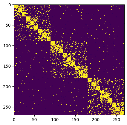
We first create a stochastic block model graph with some planted partitions at different scales.

A, coarse_scale_id, middle_scale_id, fine_scale_id = create_graph()

# Create nx graph
G = nx.from_numpy_array(A)

# Compute spring layout
pos_G = nx.layout.spring_layout(G, seed=1)


# plot matrix
plt.figure()
plt.imshow(A, interpolation="nearest")

<matplotlib.image.AxesImage at 0x125897010>

We then run pygenstability with the continuous_combinatoral constructor, which corresponds to using the combinatorial Laplacian matrix in the Markov Stability. The number and range of markov times, or scales can be specified with max_scale, min_scale and n_scales. They are in log scale by default. The number of Louvain evaluations is specified with n_tries argument.

Other options are available, see the documentation: https://barahona-research-group.github.io/PyGenStability/

# run markov stability and identify optimal scales
results = pgs.run(
    sp.csgraph.csgraph_from_dense(A),
    min_scale=-1.25,
    max_scale=0.75,
    n_scale=50,
    n_tries=20,
    constructor="continuous_combinatorial",
    n_workers=4
)

INFO:pygenstability.pygenstability:Precompute constructors...
100%|██████████████████████████████████████████████████████████████████████████████████████████████████████████████████████████████████████████████| 50/50 [00:02<00:00, 17.93it/s]
INFO:pygenstability.pygenstability:Optimise stability...
100%|██████████████████████████████████████████████████████████████████████████████████████████████████████████████████████████████████████████████| 50/50 [00:11<00:00,  4.40it/s]
INFO:pygenstability.pygenstability:Apply postprocessing...
100%|██████████████████████████████████████████████████████████████████████████████████████████████████████████████████████████████████████████████| 50/50 [00:05<00:00,  9.56it/s]
INFO:pygenstability.pygenstability:Compute ttprimes...
INFO:pygenstability.pygenstability:Identify optimal scales...

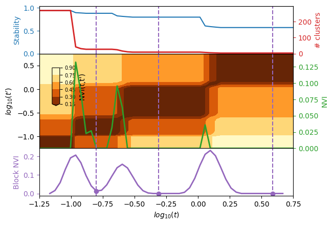
The standard plot to analyse multiscale clustering results in plot_scan, which shows various informations, such as the number of cluster, stability, normalized variation of information (NVI) between Louvain evalutions, and accros scales (NVI(t, t’)). Finally, if computed a scale selection algorithm highlights most robust scales.

# plots results
_ = plotting.plot_scan(results, figure_name=None)

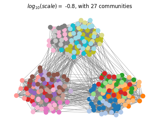
We can then plot the optimall partitions determined with the scale selection algorithm.

# plot optimal partitions
plotting.plot_optimal_partitions(G, results, show=True)

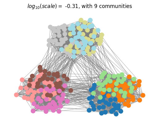
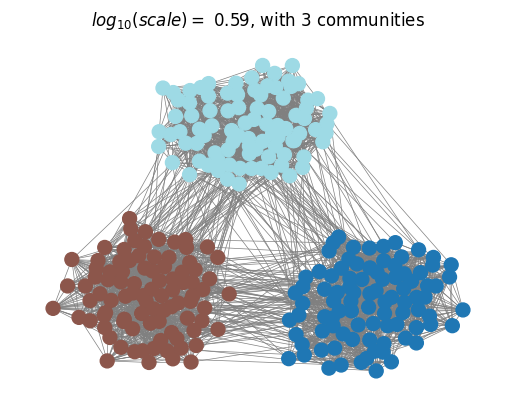
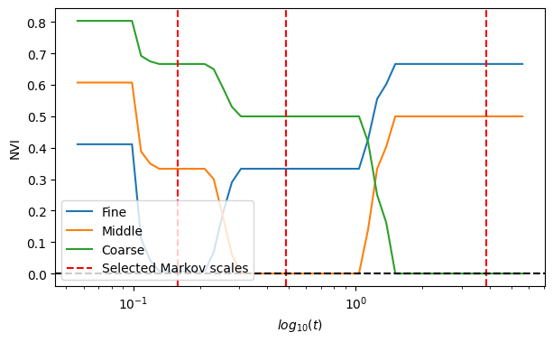
Finally, we compare the selected partitions with the ground-truth planted partitions using the Normalised Variation of Information (NVI) and observe that MS analysis with optimal scale selection recovers the planted multiscale structure of the network.

# compare MS partitions to ground truth with NVI
def _get_NVI(ref_ids):
    return [
        evaluate_NVI([0, i + 1], [ref_ids] + results["community_id"])
        for i in range(len(results["scales"]))
    ]

NVI_scores_fine = _get_NVI(fine_scale_id)
NVI_scores_middle = _get_NVI(middle_scale_id)
NVI_scores_coarse = _get_NVI(coarse_scale_id)
scales = results["scales"]

# plot NVI scores
fig, ax = plt.subplots(1, figsize=(7, 4))
ax.plot(scales, NVI_scores_fine, label="Fine")
ax.plot(scales, NVI_scores_middle, label="Middle")
ax.plot(scales, NVI_scores_coarse, label="Coarse")

# plot selected partitions
selected_partitions = results["selected_partitions"]
ax.axvline(
    x=results["scales"][selected_partitions[0]],
    ls="--",
    color="red",
    label="Selected Markov scales",
)
for i in selected_partitions[1:]:
    ax.axvline(x=results["scales"][i], ls="--", color="red")

ax.set(xlabel=r"$log_{10}(t)$", ylabel="NVI")
plt.axhline(0, c="k", ls="--")
ax.legend(loc=3)
plt.xscale("log")